5. Exploratory factor analysis and chi-square

Learning goals

You will learn to:

explain what exploratory factor analysis is for;
prepare survey items for EFA;
inspect factorability;
estimate and interpret a simple rotated factor solution;
test association between two categorical variables with chi-square.

Research questions: 1. Do the twelve survey items form the expected leadership, engagement, and role-clarity dimensions? 2. Is remote-work mode associated with high turnover intention?

Exploratory factor analysis

EFA examines whether correlations among observed items can be represented by a smaller number of latent dimensions.

It is exploratory: the pattern is learned from the data rather than fully specified in advance.

Prepare the items

library(tidyverse)
library(psych)

employees <- read_csv(
  "data/employee_survey.csv",
  show_col_types = FALSE
) |>
  mutate(
    leadership_4 = 6 - leadership_4_reverse,
    engagement_4 = 6 - engagement_4_reverse
  )

survey_items <- employees |>
  select(
    leadership_1,
    leadership_2,
    leadership_3,
    leadership_4,
    engagement_1,
    engagement_2,
    engagement_3,
    engagement_4,
    role_clarity_1,
    role_clarity_2,
    role_clarity_3,
    role_clarity_4
  ) |>
  drop_na()

For this introductory exercise, rows with missing item responses are removed. A real study should justify its missing-data strategy more carefully.

Check factorability

KMO(survey_items)

Kaiser-Meyer-Olkin factor adequacy
Call: KMO(r = survey_items)
Overall MSA =  0.9
MSA for each item = 
  leadership_1   leadership_2   leadership_3   leadership_4   engagement_1 
          0.89           0.91           0.91           0.90           0.91 
  engagement_2   engagement_3   engagement_4 role_clarity_1 role_clarity_2 
          0.92           0.92           0.89           0.88           0.91 
role_clarity_3 role_clarity_4 
          0.89           0.91

cortest.bartlett(
  cor(survey_items),
  n = nrow(survey_items)
)

$chisq
[1] 2600.465

$p.value
[1] 0

$df
[1] 66

KMO assesses whether the correlation pattern is suitable for factor analysis.
Bartlett’s test examines whether the correlation matrix differs from an identity matrix.

These diagnostics do not decide the factor solution on their own.

Explore the number of factors

fa.parallel(
  survey_items,
  fa = "fa"
)

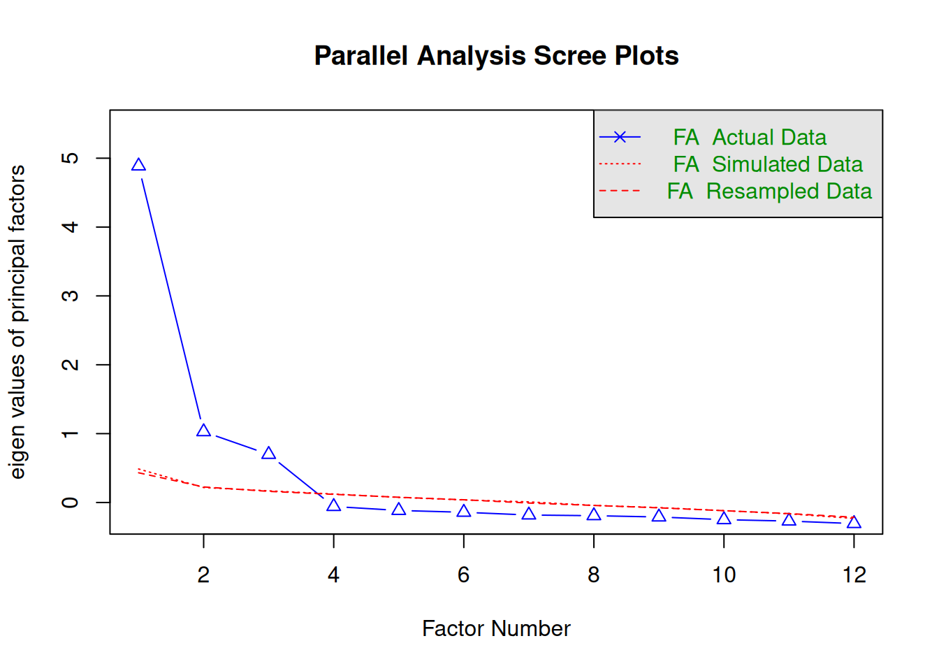
Parallel analysis suggests that the number of factors =  3  and the number of components =  NA

Parallel analysis compares observed eigenvalues with those expected from random data.

Estimate three factors

efa_model <- fa(
  survey_items,
  nfactors = 3,
  rotate = "oblimin",
  fm = "minres"
)

print(
  efa_model$loadings,
  cutoff = .30
)


Loadings:
               MR2    MR1    MR3   
leadership_1    0.853              
leadership_2    0.769              
leadership_3    0.756              
leadership_4    0.805              
engagement_1           0.769       
engagement_2           0.729       
engagement_3           0.701       
engagement_4           0.826       
role_clarity_1                0.822
role_clarity_2                0.713
role_clarity_3                0.778
role_clarity_4                0.679

                 MR2   MR1   MR3
SS loadings    2.545 2.301 2.263
Proportion Var 0.212 0.192 0.189
Cumulative Var 0.212 0.404 0.592

We use an oblique rotation because management constructs can reasonably be correlated.

A loading describes how strongly an item is related to a factor. Look for:

several meaningful loadings on each factor;
items loading strongly on their intended factor;
limited cross-loadings;
a solution that makes theoretical sense.

Chi-square test

Create categorical variables:

employees_categorical <- employees |>
  mutate(
    remote_mode = case_when(
      remote_days == 0 ~ "On-site",
      remote_days <= 3 ~ "Hybrid",
      remote_days >= 4 ~ "Mostly remote"
    ),
    high_turnover_intention = if_else(
      turnover_intention >= 5,
      "High",
      "Not high"
    )
  )

Build a contingency table:

turnover_table <- table(
  employees_categorical$remote_mode,
  employees_categorical$high_turnover_intention
)

turnover_table

               
                High Not high
  Hybrid          61      262
  Mostly remote   16       81
  On-site          9       51

prop.table(turnover_table, margin = 1)

               
                     High  Not high
  Hybrid        0.1888545 0.8111455
  Mostly remote 0.1649485 0.8350515
  On-site       0.1500000 0.8500000

Run the test:

chi_result <- chisq.test(turnover_table)

chi_result


    Pearson's Chi-squared test

data:  turnover_table
X-squared = 0.68653, df = 2, p-value = 0.7094

chi_result$expected

               
                    High  Not high
  Hybrid        57.87083 265.12917
  Mostly remote 17.37917  79.62083
  On-site       10.75000  49.25000

The chi-square test asks whether the observed combination of categories differs from what would be expected if the variables were independent.

A significant chi-square test indicates association, not the direction, magnitude, mechanism, or causality. Row percentages and a suitable effect size are needed for substantive interpretation.

Practice

Run EFA with two factors and compare the interpretability.
Identify the strongest-loading item for each factor.
Test association between department and managerial status.
Inspect expected cell counts before interpreting the chi-square result.

Common mistakes

Choosing the number of factors only because it gives a preferred result.
Treating PCA and common factor analysis as identical.
Ignoring cross-loadings and theory.
Interpreting chi-square as evidence that one category causes another.

Takeaway

EFA helps explore measurement structure; chi-square tests association between categorical variables. Both require interpretation beyond a p-value.