6. Linear regression and diagnostics

Learning goals

You will learn to:

• translate a management question into a regression model;
• interpret coefficients, confidence intervals, and model fit;
• distinguish association from causation;
• inspect linearity, residuals, multicollinearity, and influential cases;
• communicate results without overstating them.

Research question: Which marketing activities are associated with weekly sales, after accounting for the other activities and market conditions?

The idea

Linear regression estimates the expected change in a continuous outcome for a one-unit change in a predictor, while holding the other included predictors constant.

For this lesson:

• outcome: weekly sales in thousands of euros;
• predictors: search, social, and email advertising, discount, and competitor price index.

Import and inspect

library(tidyverse)
library(broom)
library(car)
library(performance)

marketing <- read_csv(
  "data/marketing_mix.csv",
  show_col_types = FALSE
)

glimpse(marketing)

Rows: 156
Columns: 8
$ week                   <dbl> 1, 2, 3, 4, 5, 6, 7, 8, 9, 10, 11, 12, 13, 14, …
$ date                   <date> 2023-01-02, 2023-01-09, 2023-01-16, 2023-01-23…
$ search_ads_k_eur       <dbl> 38.5, 42.0, 55.5, 31.6, 48.2, 48.7, 48.3, 48.8,…
$ social_ads_k_eur       <dbl> 41.0, 36.4, 53.8, 23.4, 54.7, 26.6, 34.4, 31.1,…
$ email_ads_k_eur        <dbl> 13.5, 8.6, 14.8, 9.9, 17.9, 8.5, 8.6, 15.0, 6.1…
$ discount_pct           <dbl> 7.3, 5.1, 10.5, 10.3, 5.6, 6.8, 9.0, 4.6, 5.2, …
$ competitor_price_index <dbl> 103.2, 95.0, 99.6, 100.1, 95.7, 102.7, 101.7, 1…
$ sales_k_eur            <dbl> 256.2, 255.2, 322.0, 248.2, 319.7, 270.0, 258.4…

summary(marketing)

      week             date            search_ads_k_eur social_ads_k_eur
 Min.   :  1.00   Min.   :2023-01-02   Min.   :22.80    Min.   :16.60   
 1st Qu.: 39.75   1st Qu.:2023-09-30   1st Qu.:40.92    1st Qu.:34.38   
 Median : 78.50   Median :2024-06-27   Median :47.75    Median :41.15   
 Mean   : 78.50   Mean   :2024-06-27   Mean   :47.96    Mean   :40.46   
 3rd Qu.:117.25   3rd Qu.:2025-03-25   3rd Qu.:54.33    3rd Qu.:46.60   
 Max.   :156.00   Max.   :2025-12-22   Max.   :75.00    Max.   :66.80   
 email_ads_k_eur   discount_pct    competitor_price_index  sales_k_eur   
 Min.   : 3.900   Min.   : 0.000   Min.   : 88.80         Min.   :223.9  
 1st Qu.: 9.675   1st Qu.: 6.150   1st Qu.: 96.17         1st Qu.:270.9  
 Median :11.900   Median : 8.000   Median : 99.20         Median :294.2  
 Mean   :12.042   Mean   : 7.921   Mean   : 99.29         Mean   :295.7  
 3rd Qu.:14.425   3rd Qu.: 9.850   3rd Qu.:101.62         3rd Qu.:314.4  
 Max.   :23.600   Max.   :15.200   Max.   :111.50         Max.   :420.0  

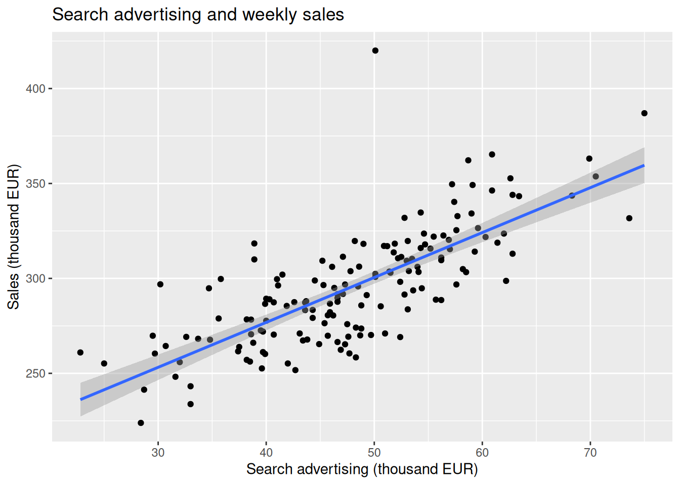
Begin with a graph

marketing |>
  ggplot(aes(x = search_ads_k_eur, y = sales_k_eur)) +
  geom_point() +
  geom_smooth(method = "lm", se = TRUE) +
  labs(
    title = "Search advertising and weekly sales",
    x = "Search advertising (thousand EUR)",
    y = "Sales (thousand EUR)"
  )

A graph is not a substitute for a model, but it can reveal nonlinearity, unusual observations, or data-entry problems.

Estimate a multiple regression

marketing_model <- lm(
  sales_k_eur ~
    search_ads_k_eur +
    social_ads_k_eur +
    email_ads_k_eur +
    discount_pct +
    competitor_price_index,
  data = marketing
)

summary(marketing_model)

Call:
lm(formula = sales_k_eur ~ search_ads_k_eur + social_ads_k_eur + 
    email_ads_k_eur + discount_pct + competitor_price_index, 
    data = marketing)

Residuals:
    Min      1Q  Median      3Q     Max 
-40.974 -12.256  -0.704  11.130 113.860 

Coefficients:
                       Estimate Std. Error t value Pr(>|t|)    
(Intercept)            271.7923    35.5800   7.639  2.4e-12 ***
search_ads_k_eur         1.9608     0.1963   9.990  < 2e-16 ***
social_ads_k_eur         0.7928     0.2030   3.905 0.000142 ***
email_ads_k_eur          1.1210     0.4037   2.777 0.006193 ** 
discount_pct             0.9138     0.4902   1.864 0.064257 .  
competitor_price_index  -1.2386     0.3463  -3.576 0.000470 ***
---
Signif. codes:  0 '***' 0.001 '**' 0.01 '*' 0.05 '.' 0.1 ' ' 1

Residual standard error: 17.85 on 150 degrees of freedom
Multiple R-squared:  0.6705,    Adjusted R-squared:  0.6595 
F-statistic: 61.04 on 5 and 150 DF,  p-value: < 2.2e-16

A compact table is easier to reuse:

tidy(marketing_model, conf.int = TRUE)

# A tibble: 6 × 7
  term                  estimate std.error statistic  p.value conf.low conf.high
  <chr>                    <dbl>     <dbl>     <dbl>    <dbl>    <dbl>     <dbl>
1 (Intercept)            272.       35.6        7.64 2.40e-12 201.       342.   
2 search_ads_k_eur         1.96      0.196      9.99 2.49e-18   1.57       2.35 
3 social_ads_k_eur         0.793     0.203      3.90 1.42e- 4   0.392      1.19 
4 email_ads_k_eur          1.12      0.404      2.78 6.19e- 3   0.323      1.92 
5 discount_pct             0.914     0.490      1.86 6.43e- 2  -0.0548     1.88 
6 competitor_price_ind…   -1.24      0.346     -3.58 4.70e- 4  -1.92      -0.554

glance(marketing_model)

# A tibble: 1 × 12
  r.squared adj.r.squared sigma statistic  p.value    df logLik   AIC   BIC
      <dbl>         <dbl> <dbl>     <dbl>    <dbl> <dbl>  <dbl> <dbl> <dbl>
1     0.670         0.659  17.9      61.0 1.93e-34     5  -668. 1350. 1371.
# ℹ 3 more variables: deviance <dbl>, df.residual <int>, nobs <int>

Interpret one coefficient

Suppose the coefficient for search_ads_k_eur is positive. The interpretation is:

Holding the other variables in the model constant, an additional thousand euros of search advertising is associated with an estimated change of b thousand euros in weekly sales.

Do not say that advertising caused the change unless the research design supports a causal conclusion.

Model fit

glance() reports, among other statistics:

• R-squared: share of sample variation in sales explained by the model;
• adjusted R-squared: R-squared adjusted for the number of predictors;
• F-test: whether the model as a whole improves on an intercept-only model.

High R-squared does not prove that the model is correct or causal.

Check multicollinearity

vif(marketing_model)

      search_ads_k_eur       social_ads_k_eur        email_ads_k_eur 
              1.780005               1.751556               1.028917 
          discount_pct competitor_price_index 
              1.020504               1.025562 

Variance inflation factors indicate whether predictors contain strongly overlapping information. They are a diagnostic signal, not an automatic rule for deleting variables.

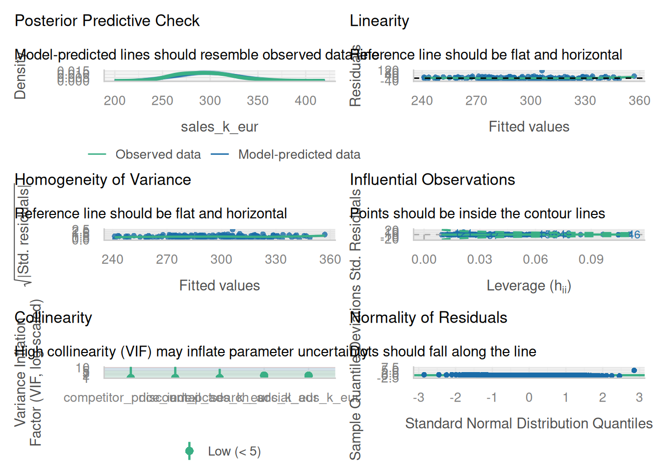
Check assumptions visually

check_model(marketing_model)

Focus on four questions:

1. Is the relationship approximately linear?
2. Are residuals distributed around zero without a clear pattern?
3. Is residual spread reasonably stable?
4. Are a few observations unusually influential?

Inspect influential observations

marketing_diagnostics <- augment(marketing_model) |>
  mutate(row_number = row_number()) |>
  arrange(desc(.cooksd))

marketing_diagnostics |>
  select(row_number, .fitted, .resid, .std.resid, .cooksd) |>
  slice_head(n = 5)

# A tibble: 5 × 5
  row_number .fitted .resid .std.resid .cooksd
       <int>   <dbl>  <dbl>      <dbl>   <dbl>
1        121    306.  114.        6.44  0.132 
2        149    334.   28.3       1.64  0.0349
3        156    357.   30.1       1.74  0.0346
4         46    277.   20.0       1.19  0.0293
5         37    304.  -34.3      -1.96  0.0230

One week in the teaching data is intentionally unusual. Investigate it rather than deleting it automatically. Ask whether it is an error, a genuine event, or evidence that the model is incomplete.

A good regression report combines the research question, coefficient estimates, uncertainty, model fit, diagnostics, and limitations. A p-value alone is not a substantive conclusion.

Practice

1. Estimate a model with only the three advertising channels.
2. Add discount and competitor price index. What changes?
3. Identify the most influential week and inspect its raw values.
4. Write a three-sentence interpretation of one coefficient.

Common mistakes

• Interpreting every coefficient causally.
• Comparing coefficient sizes when variables use very different units.
• Ignoring diagnostic plots.
• Deleting unusual observations only because they reduce significance.
• Reporting R-squared without describing the outcome and sample.

Takeaway

Regression estimates conditional associations. Credible use requires both substantive interpretation and diagnostic checking.