8. Logistic regression

Learning goals

You will learn to:

recognize when a binary outcome requires logistic regression;
estimate a beginner-friendly logistic model;
interpret odds ratios cautiously;
calculate predicted probabilities for meaningful profiles;
distinguish classification from explanation.

Research question: Which booking and guest characteristics are associated with receiving a complimentary hotel-room upgrade?

Why not linear regression?

The outcome upgrade has two values:

0: no upgrade;
1: upgrade.

Logistic regression models the log-odds of the outcome and keeps predicted probabilities between 0 and 1.

Import and prepare

library(tidyverse)
library(broom)

hotel <- read_csv(
  "data/hotel_upgrades.csv",
  show_col_types = FALSE
) |>
  mutate(
    loyalty_status = factor(
      loyalty_status,
      levels = c("None", "Silver", "Gold", "Platinum")
    ),
    special_event = factor(special_event),
    direct_booking = factor(direct_booking)
  )

Inspect the outcome:

hotel |>
  count(upgrade) |>
  mutate(percent = 100 * n / sum(n))

# A tibble: 2 × 3
  upgrade     n percent
    <dbl> <int>   <dbl>
1       0   683    75.9
2       1   217    24.1

Estimate the model

upgrade_model <- glm(
  upgrade ~
    loyalty_status +
    prior_stays +
    occupancy_rate +
    total_spend_eur +
    special_event +
    direct_booking,
  data = hotel,
  family = binomial
)

summary(upgrade_model)


Call:
glm(formula = upgrade ~ loyalty_status + prior_stays + occupancy_rate + 
    total_spend_eur + special_event + direct_booking, family = binomial, 
    data = hotel)

Coefficients:
                         Estimate Std. Error z value Pr(>|z|)    
(Intercept)            -0.0460902  0.5718317  -0.081 0.935759    
loyalty_statusSilver    0.5058974  0.2367474   2.137 0.032609 *  
loyalty_statusGold      0.6431250  0.3199056   2.010 0.044393 *  
loyalty_statusPlatinum  1.4899502  0.4898674   3.042 0.002354 ** 
prior_stays             0.1958456  0.0557478   3.513 0.000443 ***
occupancy_rate         -0.0348935  0.0069946  -4.989 6.08e-07 ***
total_spend_eur         0.0006382  0.0004254   1.500 0.133544    
special_eventYes       -0.5842472  0.2573432  -2.270 0.023189 *  
direct_bookingYes       0.5133558  0.1941297   2.644 0.008184 ** 
---
Signif. codes:  0 '***' 0.001 '**' 0.01 '*' 0.05 '.' 0.1 ' ' 1

(Dispersion parameter for binomial family taken to be 1)

    Null deviance: 994.24  on 899  degrees of freedom
Residual deviance: 798.41  on 891  degrees of freedom
AIC: 816.41

Number of Fisher Scoring iterations: 5

Convert coefficients to odds ratios

tidy(
  upgrade_model,
  exponentiate = TRUE,
  conf.int = TRUE
)

# A tibble: 9 × 7
  term                   estimate std.error statistic p.value conf.low conf.high
  <chr>                     <dbl>     <dbl>     <dbl>   <dbl>    <dbl>     <dbl>
1 (Intercept)               0.955  0.572      -0.0806 9.36e-1    0.310     2.93 
2 loyalty_statusSilver      1.66   0.237       2.14   3.26e-2    1.04      2.63 
3 loyalty_statusGold        1.90   0.320       2.01   4.44e-2    1.01      3.54 
4 loyalty_statusPlatinum    4.44   0.490       3.04   2.35e-3    1.70     11.7  
5 prior_stays               1.22   0.0557      3.51   4.43e-4    1.09      1.36 
6 occupancy_rate            0.966  0.00699    -4.99   6.08e-7    0.952     0.979
7 total_spend_eur           1.00   0.000425    1.50   1.34e-1    1.000     1.00 
8 special_eventYes          0.558  0.257      -2.27   2.32e-2    0.330     0.909
9 direct_bookingYes         1.67   0.194       2.64   8.18e-3    1.15      2.46

An odds ratio:

above 1 indicates higher estimated odds;
below 1 indicates lower estimated odds;
equal to 1 indicates no estimated change in odds.

Odds are not probabilities. An odds ratio of 2 does not mean the probability doubles.

Predicted probabilities

Predicted probabilities are often easier to communicate.

guest_profiles <- tibble(
  loyalty_status = factor(
    c("None", "Gold"),
    levels = c("None", "Silver", "Gold", "Platinum")
  ),
  prior_stays = c(0, 7),
  occupancy_rate = c(90, 65),
  total_spend_eur = c(250, 900),
  special_event = factor(
    c("No", "No"),
    levels = levels(hotel$special_event)
  ),
  direct_booking = factor(
    c("No", "Yes"),
    levels = levels(hotel$direct_booking)
  )
)

guest_profiles |>
  mutate(
    predicted_probability = predict(
      upgrade_model,
      newdata = guest_profiles,
      type = "response"
    )
  )

# A tibble: 2 × 7
  loyalty_status prior_stays occupancy_rate total_spend_eur special_event
  <fct>                <dbl>          <dbl>           <dbl> <fct>        
1 None                     0             90             250 No           
2 Gold                     7             65             900 No           
# ℹ 2 more variables: direct_booking <fct>, predicted_probability <dbl>

The two profiles differ on several characteristics, so this comparison is a scenario illustration rather than the isolated effect of one variable.

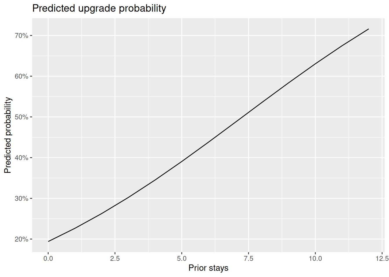
A one-variable probability plot

probability_data <- tibble(
  loyalty_status = factor(
    "Silver",
    levels = c("None", "Silver", "Gold", "Platinum")
  ),
  prior_stays = 0:12,
  occupancy_rate = mean(hotel$occupancy_rate),
  total_spend_eur = median(hotel$total_spend_eur),
  special_event = factor(
    "No", levels = levels(hotel$special_event)
  ),
  direct_booking = factor(
    "Yes", levels = levels(hotel$direct_booking)
  )
)

probability_data <- probability_data |>
  mutate(
    probability = predict(
      upgrade_model,
      newdata = probability_data,
      type = "response"
    )
  )

probability_data |>
  ggplot(aes(x = prior_stays, y = probability)) +
  geom_line() +
  scale_y_continuous(labels = scales::percent) +
  labs(
    title = "Predicted upgrade probability",
    x = "Prior stays",
    y = "Predicted probability"
  )

Practice

Fit a smaller model using loyalty, occupancy, and direct booking.
Compare odds ratios with predicted probabilities.
Create two profiles that differ only in loyalty status.
Explain why a predictive association may not represent a fair decision rule.

Common mistakes

Interpreting odds ratios as probabilities.
Treating a significant predictor as a causal driver.
Reporting accuracy without considering class balance.
Using sensitive or proxy variables without ethical reflection.
Assuming a simulated teaching model is suitable for deployment.

Takeaway

Logistic regression models binary outcomes. Predicted probabilities usually provide the clearest applied interpretation, but ethical and design questions remain essential.