Solutions: Exercises 3–4

library(tidyverse)
library(effectsize)
library(psych)

employees <- read_csv("data/employee_survey.csv", show_col_types = FALSE)

cor.test(employees$workload, employees$burnout)


    Pearson's product-moment correlation

data:  employees$workload and employees$burnout
t = 19.429, df = 478, p-value < 2.2e-16
alternative hypothesis: true correlation is not equal to 0
95 percent confidence interval:
 0.6111010 0.7114717
sample estimates:
    cor 
0.66427

t_result <- t.test(performance ~ training_group, data = employees)
t_result


    Welch Two Sample t-test

data:  performance by training_group
t = -4.3995, df = 463.73, p-value = 1.347e-05
alternative hypothesis: true difference in means between group Control and group Training is not equal to 0
95 percent confidence interval:
 -5.270074 -2.015756
sample estimates:
 mean in group Control mean in group Training 
              51.96728               55.61020

cohens_d(performance ~ training_group, data = employees)

Cohen's d |         95% CI
--------------------------
-0.40     | [-0.59, -0.22]

- Estimated using pooled SD.

experiment <- read_csv("data/training_experiment.csv", show_col_types = FALSE)
t.test(post_score ~ group, data = experiment)


    Welch Two Sample t-test

data:  post_score by group
t = -2.3536, df = 217.85, p-value = 0.01948
alternative hypothesis: true difference in means between group Control and group Training is not equal to 0
95 percent confidence interval:
 -6.2358887 -0.5517717
sample estimates:
 mean in group Control mean in group Training 
              65.10522               68.49905

t.test(
  experiment$post_score[experiment$group == "Training"],
  experiment$pre_score[experiment$group == "Training"],
  paired = TRUE
)


    Paired t-test

data:  experiment$post_score[experiment$group == "Training"] and experiment$pre_score[experiment$group == "Training"]
t = 19.965, df = 104, p-value < 2.2e-16
alternative hypothesis: true mean difference is not equal to 0
95 percent confidence interval:
 6.501155 7.935035
sample estimates:
mean difference 
       7.218095

employees <- employees |>
  mutate(
    leadership_4 = 6 - leadership_4_reverse,
    engagement_4 = 6 - engagement_4_reverse,
    leadership = rowMeans(
      across(c(leadership_1, leadership_2, leadership_3, leadership_4)),
      na.rm = TRUE
    ),
    engagement = rowMeans(
      across(c(engagement_1, engagement_2, engagement_3, engagement_4)),
      na.rm = TRUE
    )
  )

alpha(employees |> select(starts_with("leadership_") & !ends_with("reverse")))


Reliability analysis   
Call: alpha(x = select(employees, starts_with("leadership_") & !ends_with("reverse")))

  raw_alpha std.alpha G6(smc) average_r S/N    ase mean  sd median_r
      0.87      0.87    0.84      0.63 6.8 0.0095    3 1.2     0.64

    95% confidence boundaries 
         lower alpha upper
Feldt     0.85  0.87  0.89
Duhachek  0.85  0.87  0.89

 Reliability if an item is dropped:
             raw_alpha std.alpha G6(smc) average_r S/N alpha se   var.r med.r
leadership_1      0.82      0.82    0.76      0.60 4.6    0.014 0.00152  0.63
leadership_2      0.84      0.84    0.78      0.65 5.5    0.012 0.00032  0.65
leadership_3      0.85      0.85    0.79      0.65 5.6    0.012 0.00034  0.66
leadership_4      0.83      0.83    0.77      0.62 4.9    0.013 0.00290  0.65

 Item statistics 
               n raw.r std.r r.cor r.drop mean  sd
leadership_1 480  0.87  0.87  0.82   0.76  3.0 1.3
leadership_2 472  0.84  0.84  0.76   0.71  3.0 1.4
leadership_3 480  0.83  0.83  0.75   0.70  3.0 1.4
leadership_4 472  0.86  0.86  0.79   0.74  2.9 1.4

Non missing response frequency for each item
                1    2    3    4    5 miss
leadership_1 0.17 0.22 0.23 0.20 0.18 0.00
leadership_2 0.20 0.21 0.21 0.19 0.19 0.02
leadership_3 0.19 0.22 0.21 0.19 0.19 0.00
leadership_4 0.19 0.22 0.24 0.17 0.18 0.02

items <- employees |>
  select(
    leadership_1, leadership_2, leadership_3, leadership_4,
    engagement_1, engagement_2, engagement_3, engagement_4,
    role_clarity_1, role_clarity_2, role_clarity_3, role_clarity_4
  ) |>
  drop_na()

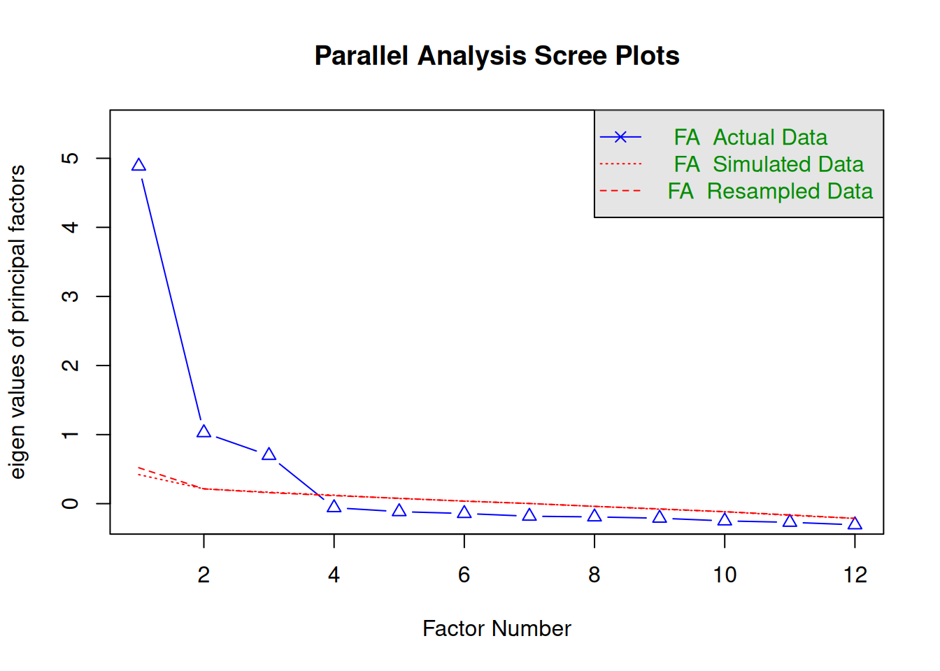
fa.parallel(items, fa = "fa")

Parallel analysis suggests that the number of factors =  3  and the number of components =  NA

efa <- fa(items, nfactors = 3, rotate = "oblimin", fm = "minres")
print(efa$loadings, cutoff = .30)


Loadings:
               MR2    MR3    MR1   
leadership_1    0.853              
leadership_2    0.769              
leadership_3    0.756              
leadership_4    0.805              
engagement_1           0.769       
engagement_2           0.729       
engagement_3           0.701       
engagement_4           0.826       
role_clarity_1                0.822
role_clarity_2                0.713
role_clarity_3                0.778
role_clarity_4                0.679

                 MR2   MR3   MR1
SS loadings    2.545 2.301 2.263
Proportion Var 0.212 0.192 0.189
Cumulative Var 0.212 0.404 0.592

manager_department <- table(employees$manager, employees$department)
chisq.test(manager_department)


    Pearson's Chi-squared test

data:  manager_department
X-squared = 5.4999, df = 4, p-value = 0.2397