10. Nested data and multilevel models

Learning goals

You will learn to:

recognize nested or clustered management data;
explain why observations within a team may not be independent;
distinguish Level 1 from Level 2 variables;
calculate the intuition behind the intraclass correlation coefficient (ICC);
fit a random-intercept model with lme4;
explain what multilevel modelling changes relative to an ordinary regression.

Management question: Employee performance may depend on individual engagement and workload, but employees work inside teams that differ in climate and manager support. How should we analyse both levels at once?

Management data are often nested

EmployeesinsideTeamsinsideBusiness units

Other examples:

repeated monthly observations inside stores;
employees inside departments;
branches inside regions;
transactions inside customers;
survey waves inside the same person.

When observations share a context, they can be more similar than randomly selected observations.

Why ordinary regression can be incomplete

Standard linear regression assumes, among other things, that residual information is independent across observations.

If employees in the same team share a manager, routines, climate, and local shocks, treating all 600 employees as unrelated can underestimate or otherwise misrepresent uncertainty.

Multilevel models represent this structure explicitly.

The dataset

library(tidyverse)
library(lme4)

teams <- read_csv(
  "data/multilevel_teams.csv",
  show_col_types = FALSE
)

glimpse(teams)

Rows: 600
Columns: 11
$ employee_id     <chr> "E0001", "E0002", "E0003", "E0004", "E0005", "E0006", …
$ team_id         <chr> "T01", "T01", "T01", "T01", "T01", "T01", "T01", "T01"…
$ business_unit   <chr> "Consumer", "Consumer", "Consumer", "Consumer", "Consu…
$ age             <dbl> 42, 34, 34, 39, 49, 24, 39, 44, 37, 35, 22, 25, 24, 29…
$ tenure_years    <dbl> 3.5, 3.9, 4.2, 2.7, 9.8, 2.0, 5.7, 5.3, 13.3, 8.4, 2.4…
$ autonomy        <dbl> 4.54, 4.64, 4.03, 4.64, 4.49, 5.96, 5.56, 4.58, 5.96, …
$ workload        <dbl> 4.09, 4.72, 3.50, 5.69, 2.74, 3.91, 6.29, 3.38, 3.39, …
$ engagement      <dbl> 5.06, 4.57, 5.88, 4.70, 4.63, 6.37, 2.41, 5.73, 4.89, …
$ team_climate    <dbl> 4.83, 4.83, 4.83, 4.83, 4.83, 4.83, 4.83, 4.83, 4.83, …
$ manager_support <dbl> 5.67, 5.67, 5.67, 5.67, 5.67, 5.67, 5.67, 5.67, 5.67, …
$ performance     <dbl> 83.3, 69.7, 84.5, 66.6, 78.3, 92.6, 65.9, 83.6, 79.3, …

teams |>
  count(team_id) |>
  summarise(
    teams = n(),
    min_members = min(n),
    max_members = max(n)
  )

# A tibble: 1 × 3
  teams min_members max_members
  <int>       <int>       <int>
1    50          12          12

The file has 600 employees nested in 50 teams.

Identify levels

Level 1 — employee

engagement
autonomy
workload
age
tenure
performance

Level 2 — team

team climate
manager support
team identifier

Team-level variables repeat for every employee in the same team because they describe the shared context.

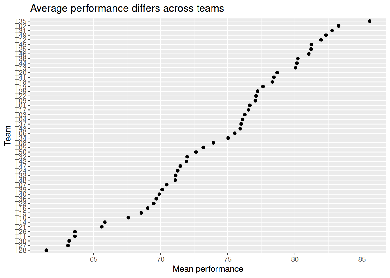
Visualize team differences

teams |>
  group_by(team_id) |>
  summarise(
    mean_performance = mean(performance),
    .groups = "drop"
  ) |>
  ggplot(aes(x = reorder(team_id, mean_performance), y = mean_performance)) +
  geom_point() +
  coord_flip() +
  labs(
    title = "Average performance differs across teams",
    x = "Team",
    y = "Mean performance"
  )

Start with the empty model

empty_model <- lmer(
  performance ~ 1 + (1 | team_id),
  data = teams,
  REML = TRUE
)

summary(empty_model)

Linear mixed model fit by REML ['lmerMod']
Formula: performance ~ 1 + (1 | team_id)
   Data: teams

REML criterion at convergence: 4390.9

Scaled residuals: 
    Min      1Q  Median      3Q     Max 
-3.4040 -0.6456  0.0145  0.6526  3.1467 

Random effects:
 Groups   Name        Variance Std.Dev.
 team_id  (Intercept) 30.35    5.509   
 Residual             76.61    8.753   
Number of obs: 600, groups:  team_id, 50

Fixed effects:
            Estimate Std. Error t value
(Intercept)  74.0373     0.8572   86.37

(1 | team_id) means: allow each team to have its own intercept around an overall average.

Intraclass correlation (ICC)

The ICC answers:

What share of unexplained variance in performance lies between teams rather than within teams?

variance_parts <- as.data.frame(
  VarCorr(empty_model)
)

team_variance <- variance_parts$vcov[
  variance_parts$grp == "team_id"
][1]

residual_variance <- sigma(empty_model)^2

icc <- team_variance /
  (team_variance + residual_variance)

icc

[1] 0.2837703

An ICC near zero means little clustering by team. A larger ICC means employees in the same team are more similar on the outcome.

The ICC is descriptive evidence about clustering; it is not a universal threshold that automatically chooses a model.

Add employee- and team-level predictors

multilevel_model <- lmer(
  performance ~
    engagement +
    autonomy +
    workload +
    team_climate +
    manager_support +
    (1 | team_id),
  data = teams,
  REML = TRUE
)

summary(multilevel_model)

Linear mixed model fit by REML ['lmerMod']
Formula: performance ~ engagement + autonomy + workload + team_climate +  
    manager_support + (1 | team_id)
   Data: teams

REML criterion at convergence: 4015.9

Scaled residuals: 
    Min      1Q  Median      3Q     Max 
-3.1894 -0.6173 -0.0045  0.6118  2.6773 

Random effects:
 Groups   Name        Variance Std.Dev.
 team_id  (Intercept) 23.80    4.879   
 Residual             40.35    6.352   
Number of obs: 600, groups:  team_id, 50

Fixed effects:
                Estimate Std. Error t value
(Intercept)      39.1783     7.1389   5.488
engagement        4.5782     0.3489  13.123
autonomy          1.9336     0.3002   6.440
workload         -2.6658     0.2785  -9.572
team_climate     -0.4102     1.1913  -0.344
manager_support   3.3436     1.4258   2.345

Correlation of Fixed Effects:
            (Intr) enggmn autnmy workld tm_clm
engagement  -0.128                            
autonomy    -0.065 -0.409                     
workload    -0.176  0.286 -0.197              
team_climat -0.298 -0.086  0.008 -0.004       
mangr_spprt -0.647 -0.011 -0.002 -0.022 -0.476

Now the model contains:

fixed effects for average relationships;
a random team intercept for unobserved team-to-team differences.

Compare with a naive regression

naive_model <- lm(
  performance ~
    engagement +
    autonomy +
    workload +
    team_climate +
    manager_support,
  data = teams
)

coef(summary(naive_model))

                  Estimate Std. Error   t value     Pr(>|t|)
(Intercept)     38.9787383  3.6824357 10.585042 4.192815e-24
engagement       4.6727621  0.4232628 11.039859 6.654828e-26
autonomy         1.8334932  0.3608835  5.080568 5.046686e-07
workload        -2.5971246  0.3311868 -7.841871 2.067436e-14
team_climate    -0.4257966  0.5381656 -0.791200 4.291431e-01
manager_support  3.3371647  0.6275995  5.317347 1.492766e-07

coef(summary(multilevel_model))

                  Estimate Std. Error    t value
(Intercept)     39.1782650  7.1389129  5.4879876
engagement       4.5782124  0.3488634 13.1232254
autonomy         1.9336050  0.3002481  6.4400241
workload        -2.6658346  0.2784960 -9.5722553
team_climate    -0.4101585  1.1912539 -0.3443082
manager_support  3.3436041  1.4257903  2.3450883

Do not compare only coefficients. Pay attention to standard errors and uncertainty, because clustering particularly affects inference.

Optional next step: random slopes

Sometimes the engagement–performance relationship itself differs between teams.

random_slope_model <- lmer(
  performance ~
    engagement +
    autonomy +
    workload +
    team_climate +
    manager_support +
    (1 + engagement | team_id),
  data = teams
)

Random slopes are powerful but require more data and more diagnostic attention, so they are an extension rather than the beginner default.

Centering: why you will see it later

In multilevel research, researchers often distinguish:

within-team differences: is an employee more engaged than teammates?
between-team differences: are some teams more engaged on average?

Centering and decomposition help separate these questions. The choice should follow the substantive theory.

A multilevel model is not merely “a more advanced regression.” It represents a claim about the structure of the data-generating context.

Practice

Count employees per team.
Fit the empty random-intercept model.
Calculate the ICC.
Fit the full multilevel model.
Identify one employee-level and one team-level coefficient.
Compare standard errors with the ordinary regression.
Explain why 600 employees in 50 teams are not the same design as 600 independent employees.

Takeaway

When management data are nested or repeated, the unit of observation is not the whole design. Multilevel analysis lets us model individual relationships while respecting shared organizational context.

References

Bates, Mächler, Bolker & Walker (2015), Fitting Linear Mixed-Effects Models Using lme4, Journal of Statistical Software. https://doi.org/10.18637/jss.v067.i01
lme4 documentation and vignette
Schonfeld & Rindskopf (2007), Hierarchical Linear Modeling in Organizational Research, Organizational Research Methods. https://doi.org/10.1177/1094428107300229