11. Scenario-based management analysis: diagnosing stagnant sales

Learning goals

You will learn to:

turn a managerial problem into a structured analytical case;
distinguish diagnosis, prediction, scenario analysis, and causal inference;
build a transparent regression-based what-if model;
create alternative management scenarios with newdata;
compare predicted outcomes without presenting scenarios as proven interventions;
recognize repeated branch observations as a multilevel issue.

Management situation: Marketing spending has been rising, but sales appear stagnant. Senior management asks: “What is holding sales back, and what could happen under different operational scenarios?”

The decision problem

Scenario analysis is useful when management needs to compare plausible combinations of assumptions rather than pretend there is one certain forecast.

Diagnose→Model→Define scenarios→Compare→Stress-test interpretation

The dataset

library(tidyverse)
library(broom)

retail <- read_csv(
  "data/stagnant_retail.csv",
  show_col_types = FALSE
)

glimpse(retail)

Rows: 288
Columns: 11
$ branch_id           <chr> "B01", "B01", "B01", "B01", "B01", "B01", "B01", "…
$ region              <chr> "North", "North", "North", "North", "North", "Nort…
$ month               <date> 2025-01-01, 2025-02-01, 2025-03-01, 2025-04-01, 2…
$ month_number        <dbl> 1, 2, 3, 4, 5, 6, 7, 8, 9, 10, 11, 12, 1, 2, 3, 4,…
$ sales_k_eur         <dbl> 425.3, 402.2, 384.9, 380.9, 377.6, 381.5, 369.1, 3…
$ footfall_k          <dbl> 20.02, 18.32, 15.75, 15.70, 16.70, 17.67, 15.37, 1…
$ marketing_k_eur     <dbl> 20.20, 22.49, 24.15, 27.38, 28.79, 27.85, 25.22, 2…
$ discount_pct        <dbl> 11.79, 10.24, 9.96, 12.82, 7.69, 6.62, 8.05, 12.16…
$ service_quality     <dbl> 4.53, 4.37, 4.49, 4.55, 4.74, 4.54, 4.61, 4.40, 4.…
$ competitor_pressure <dbl> 0.319, 0.385, 0.384, 0.458, 0.422, 0.474, 0.560, 0…
$ conversion_rate     <dbl> 0.268, 0.265, 0.272, 0.265, 0.265, 0.248, 0.284, 0…

The dataset contains 24 synthetic branches observed monthly for 12 months.

Key variables:

sales;
footfall;
marketing spend;
discount;
service quality;
competitor pressure;
conversion rate.

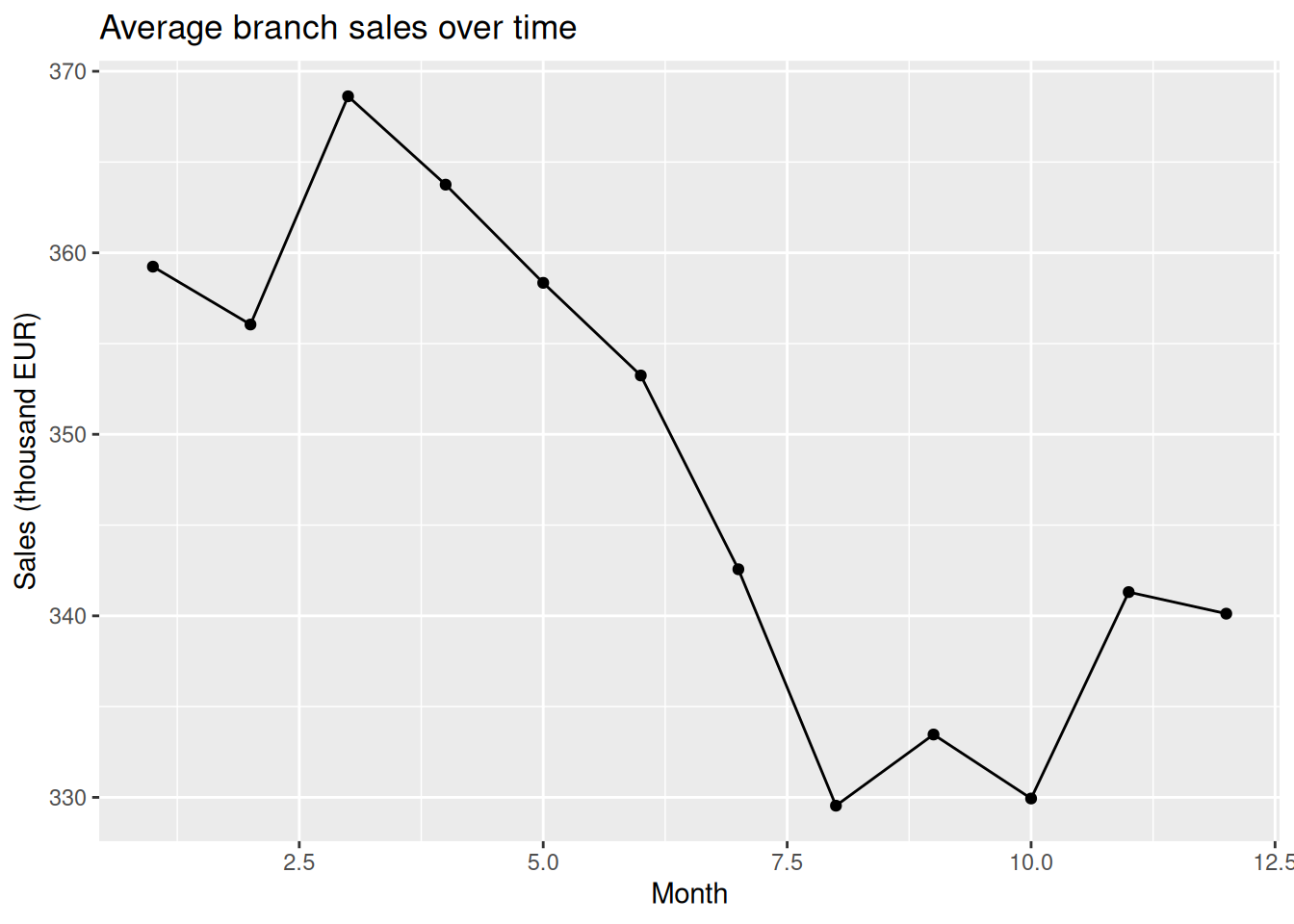
Is sales really stagnant?

Aggregate by month:

monthly <- retail |>
  group_by(month_number) |>
  summarise(
    sales = mean(sales_k_eur),
    marketing = mean(marketing_k_eur),
    footfall = mean(footfall_k),
    competitor_pressure = mean(competitor_pressure),
    .groups = "drop"
  )

monthly

# A tibble: 12 × 5
   month_number sales marketing footfall competitor_pressure
          <dbl> <dbl>     <dbl>    <dbl>               <dbl>
 1            1  359.      20.8     15.5               0.349
 2            2  356.      21.3     15.5               0.377
 3            3  369.      22.7     15.5               0.385
 4            4  364.      22.9     15.1               0.412
 5            5  358.      24.1     15.2               0.429
 6            6  353.      25.2     14.7               0.470
 7            7  343.      24.5     14.6               0.483
 8            8  330.      26.2     13.9               0.495
 9            9  333.      26.7     14.0               0.498
10           10  330.      27.2     13.7               0.510
11           11  341.      28.6     14.0               0.543
12           12  340.      29.7     13.4               0.542

Plot sales and marketing separately:

ggplot(monthly, aes(x = month_number, y = sales)) +
  geom_line() +
  geom_point() +
  labs(
    title = "Average branch sales over time",
    x = "Month",
    y = "Sales (thousand EUR)"
  )

ggplot(monthly, aes(x = month_number, y = marketing)) +
  geom_line() +
  geom_point() +
  labs(
    title = "Average marketing spend over time",
    x = "Month",
    y = "Marketing spend (thousand EUR)"
  )

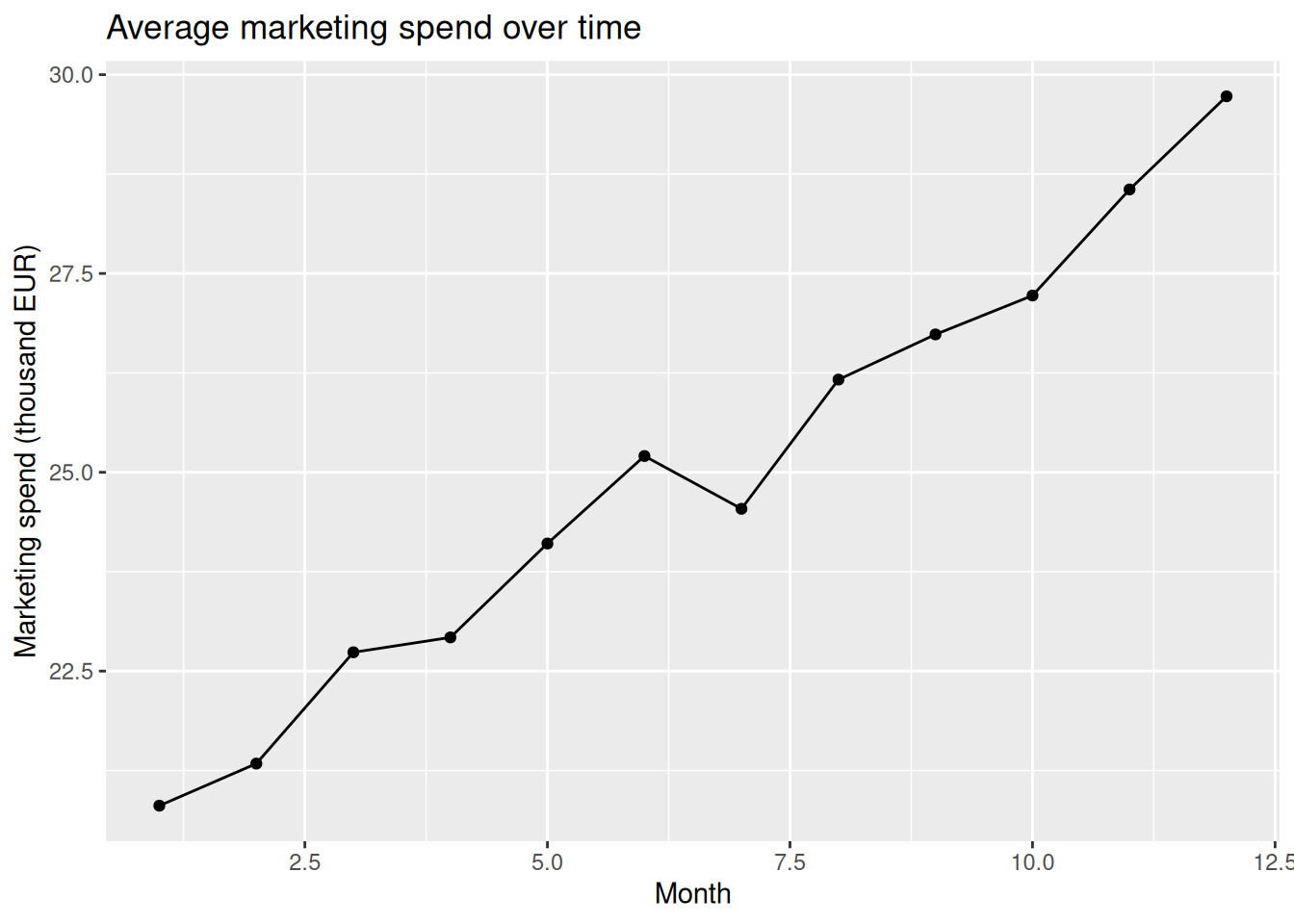
A useful managerial question emerges: if marketing increased but sales did not rise proportionally, what else changed?

Explore candidate explanations

retail |>
  summarise(
    cor_sales_footfall = cor(sales_k_eur, footfall_k),
    cor_sales_marketing = cor(sales_k_eur, marketing_k_eur),
    cor_sales_competition = cor(sales_k_eur, competitor_pressure)
  )

# A tibble: 1 × 3
  cor_sales_footfall cor_sales_marketing cor_sales_competition
               <dbl>               <dbl>                 <dbl>
1              0.798              -0.223                -0.353

These correlations are diagnostic clues, not causal estimates.

Build a transparent working model

scenario_model <- lm(
  sales_k_eur ~
    footfall_k +
    marketing_k_eur +
    discount_pct +
    service_quality +
    competitor_pressure +
    conversion_rate,
  data = retail
)

tidy(
  scenario_model,
  conf.int = TRUE
)

# A tibble: 7 × 7
  term                estimate std.error statistic  p.value conf.low conf.high
  <chr>                  <dbl>     <dbl>     <dbl>    <dbl>    <dbl>     <dbl>
1 (Intercept)          113.       12.7        8.88 8.20e-17   87.7      138.  
2 footfall_k            10.2       0.449     22.6  2.71e-65    9.27      11.0 
3 marketing_k_eur        0.930     0.306      3.04 2.58e- 3    0.328      1.53
4 discount_pct           2.70      0.406      6.66 1.45e-10    1.90       3.50
5 service_quality        9.30      1.81       5.15 4.86e- 7    5.75      12.9 
6 competitor_pressure  -92.8      14.1       -6.60 2.06e-10 -121.       -65.1 
7 conversion_rate      189.       28.0        6.77 7.50e-11  134.       244.

The purpose here is not to claim a final causal model. It is to create a transparent relationship model for structured what-if analysis.

Define a baseline

baseline <- retail |>
  summarise(
    footfall_k = median(footfall_k),
    marketing_k_eur = median(marketing_k_eur),
    discount_pct = median(discount_pct),
    service_quality = median(service_quality),
    competitor_pressure = median(competitor_pressure),
    conversion_rate = median(conversion_rate)
  )

Create management scenarios

scenarios <- bind_rows(
  baseline |>
    mutate(scenario = "Baseline"),

  baseline |>
    mutate(
      marketing_k_eur = marketing_k_eur * 1.15,
      scenario = "Marketing +15%"
    ),

  baseline |>
    mutate(
      service_quality = pmin(service_quality + 0.4, 5),
      scenario = "Service +0.4"
    ),

  baseline |>
    mutate(
      marketing_k_eur = marketing_k_eur * 1.15,
      service_quality = pmin(service_quality + 0.4, 5),
      scenario = "Marketing +15% & service +0.4"
    ),

  baseline |>
    mutate(
      competitor_pressure = pmin(competitor_pressure + 0.05, 1),
      scenario = "Competitor pressure +0.05"
    )
)

Predict the model under each scenario

scenario_predictions <- predict(
  scenario_model,
  newdata = scenarios,
  interval = "confidence"
) |>
  as.data.frame()

scenario_results <- bind_cols(
  scenarios,
  scenario_predictions
) |>
  select(
    scenario,
    fit,
    lwr,
    upr,
    everything()
  )

scenario_results

# A tibble: 5 × 10
  scenario               fit   lwr   upr footfall_k marketing_k_eur discount_pct
  <chr>                <dbl> <dbl> <dbl>      <dbl>           <dbl>        <dbl>
1 Baseline              347.  346.  349.       14.6            25.0         9.44
2 Marketing +15%        351.  348.  354.       14.6            28.7         9.44
3 Service +0.4          351.  349.  354.       14.6            25.0         9.44
4 Marketing +15% & se…  355.  352.  358.       14.6            28.7         9.44
5 Competitor pressure…  343.  341.  345.       14.6            25.0         9.44
# ℹ 3 more variables: service_quality <dbl>, competitor_pressure <dbl>,
#   conversion_rate <dbl>

The columns fit, lwr, and upr are model-based predictions and confidence bounds for the expected mean response under the specified predictor combinations.

The most important interpretation rule

Changing marketing_k_eur in newdata does not prove what would causally happen if management increased marketing by 15%. It asks: what does this fitted model predict at that combination of inputs?

Scenario analysis is especially useful for:

comparing assumptions;
exposing trade-offs;
asking “what would need to be true?”;
identifying variables worth investigating further;
communicating uncertainty.

It is not a substitute for experiments, causal identification, or a defensible forecasting design.

An organizational complication: repeated branches

Each branch appears 12 times.

That means the observations are nested/repeated within branch. For a more defensible inferential model, connect this lesson to Nested data and multilevel models.

A management conclusion template

A careful conclusion might say:

Sales remained comparatively flat while marketing expenditure increased. The working model associates sales more strongly with a combination of footfall, conversion, service quality, and competitive pressure than with marketing expenditure alone. Scenario predictions suggest where management could focus further investigation, but they should not be interpreted as causal intervention effects.

Practice

Plot average sales, marketing, footfall, and competitor pressure across months.
Fit the working regression.
Create a “Discount +3 percentage points” scenario.
Create a “Footfall -5%” stress scenario.
Compare model predictions.
Write a 100-word note to management distinguishing diagnosis, scenario prediction, and causal evidence.

Takeaway

Good scenario analysis makes assumptions explicit. R helps us calculate consistent what-if comparisons; management judgment and research design determine how seriously those comparisons should be treated.

Reference

R documentation: predict.lm()