library(tidyverse)
library(broom)
library(car)
library(performance)
library(interactions)
library(mediation)

marketing <- read_csv("data/marketing_mix.csv", show_col_types = FALSE)

model_1 <- lm(
  sales_k_eur ~ search_ads_k_eur + social_ads_k_eur + email_ads_k_eur,
  data = marketing
)
model_2 <- update(
  model_1,
  . ~ . + discount_pct + competitor_price_index
)

glance(model_1) |> dplyr::select(r.squared, adj.r.squared)
# A tibble: 1 × 2
r.squared adj.r.squared
<dbl> <dbl>
1 0.636 0.628# A tibble: 1 × 2
r.squared adj.r.squared
<dbl> <dbl>
1 0.670 0.659tidy(model_2, conf.int = TRUE)# A tibble: 6 × 7
term estimate std.error statistic p.value conf.low conf.high
<chr> <dbl> <dbl> <dbl> <dbl> <dbl> <dbl>
1 (Intercept) 272. 35.6 7.64 2.40e-12 201. 342.
2 search_ads_k_eur 1.96 0.196 9.99 2.49e-18 1.57 2.35
3 social_ads_k_eur 0.793 0.203 3.90 1.42e- 4 0.392 1.19
4 email_ads_k_eur 1.12 0.404 2.78 6.19e- 3 0.323 1.92
5 discount_pct 0.914 0.490 1.86 6.43e- 2 -0.0548 1.88
6 competitor_price_ind… -1.24 0.346 -3.58 4.70e- 4 -1.92 -0.554vif(model_2) search_ads_k_eur social_ads_k_eur email_ads_k_eur
1.780005 1.751556 1.028917
discount_pct competitor_price_index
1.020504 1.025562 check_model(model_2)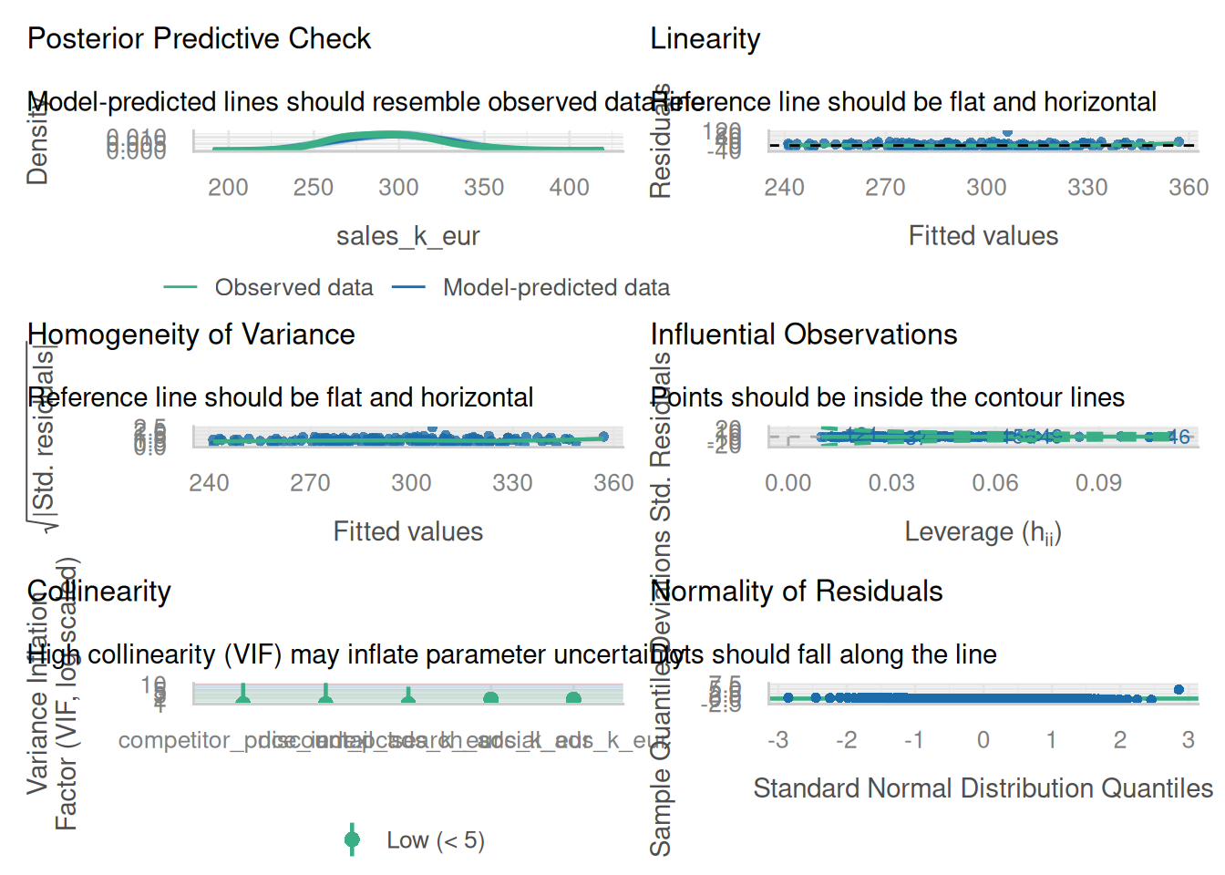
augmented <- augment(model_2) |> mutate(row_number = row_number())
most_influential <- augmented |> slice_max(.cooksd, n = 1)
most_influential
# A tibble: 1 × 13
sales_k_eur search_ads_k_eur social_ads_k_eur email_ads_k_eur discount_pct
<dbl> <dbl> <dbl> <dbl> <dbl>
1 420 50.1 38.6 14.7 7.6
# ℹ 8 more variables: competitor_price_index <dbl>, .fitted <dbl>,
# .resid <dbl>, .hat <dbl>, .sigma <dbl>, .cooksd <dbl>, .std.resid <dbl>,
# row_number <int># A tibble: 12 × 6
term estimate std.error statistic p.value model
<chr> <dbl> <dbl> <dbl> <dbl> <chr>
1 (Intercept) 272. 35.6 7.64 2.40e-12 All weeks
2 search_ads_k_eur 1.96 0.196 9.99 2.49e-18 All weeks
3 social_ads_k_eur 0.793 0.203 3.90 1.42e- 4 All weeks
4 email_ads_k_eur 1.12 0.404 2.78 6.19e- 3 All weeks
5 discount_pct 0.914 0.490 1.86 6.43e- 2 All weeks
6 competitor_price_index -1.24 0.346 -3.58 4.70e- 4 All weeks
7 (Intercept) 256. 30.4 8.40 3.20e-14 Sensitivity
8 search_ads_k_eur 1.89 0.168 11.3 1.13e-21 Sensitivity
9 social_ads_k_eur 0.854 0.173 4.92 2.25e- 6 Sensitivity
10 email_ads_k_eur 0.966 0.345 2.80 5.84e- 3 Sensitivity
11 discount_pct 0.930 0.418 2.22 2.78e- 2 Sensitivity
12 competitor_price_index -1.06 0.297 -3.57 4.86e- 4 Sensitivityemployees <- read_csv("data/employee_survey.csv", show_col_types = FALSE) |>
mutate(
leadership_4 = 6 - leadership_4_reverse,
engagement_4 = 6 - engagement_4_reverse,
leadership = rowMeans(across(c(leadership_1, leadership_2, leadership_3, leadership_4)), na.rm = TRUE),
engagement = rowMeans(across(c(engagement_1, engagement_2, engagement_3, engagement_4)), na.rm = TRUE),
workload_c = workload - mean(workload, na.rm = TRUE),
support_c = organizational_support - mean(organizational_support, na.rm = TRUE)
)
moderation_model <- lm(
burnout ~ workload_c * support_c + age + tenure_years,
data = employees
)
tidy(moderation_model, conf.int = TRUE)# A tibble: 6 × 7
term estimate std.error statistic p.value conf.low conf.high
<chr> <dbl> <dbl> <dbl> <dbl> <dbl> <dbl>
1 (Intercept) 42.0 1.34 31.4 4.77e-118 39.4 44.6
2 workload_c 6.11 0.279 21.9 5.32e- 74 5.57 6.66
3 support_c -3.37 0.301 -11.2 4.92e- 26 -3.97 -2.78
4 age 0.0475 0.0321 1.48 1.39e- 1 -0.0155 0.111
5 tenure_years 0.155 0.0818 1.90 5.83e- 2 -0.00545 0.316
6 workload_c:support_c -2.12 0.303 -6.98 9.71e- 12 -2.71 -1.52 interact_plot(moderation_model, pred = workload_c, modx = support_c)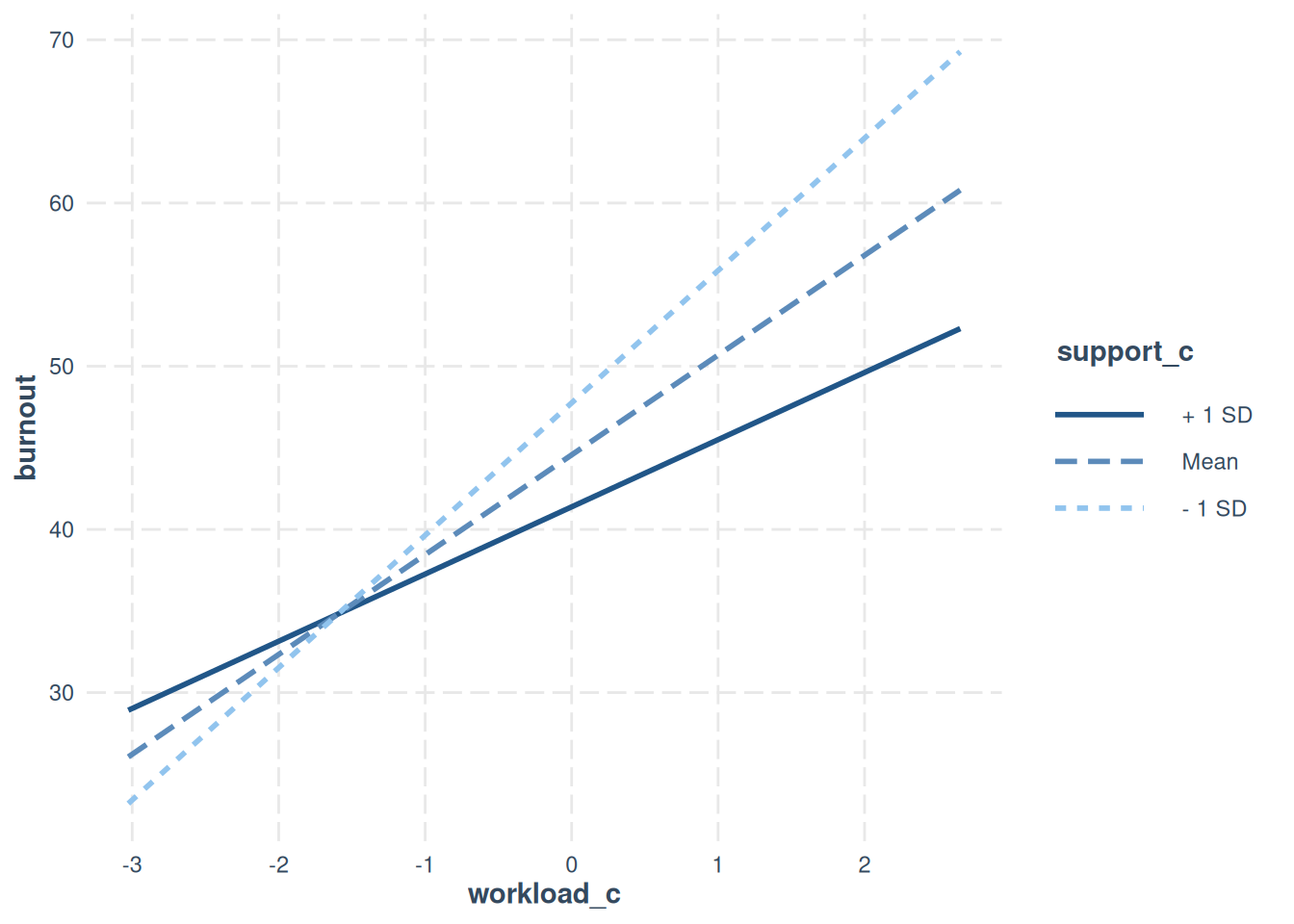
mediation_data <- employees |>
  drop_na(leadership, engagement, performance, age, tenure_years)

mediator_model <- lm(engagement ~ leadership + age + tenure_years, data = mediation_data)
outcome_model <- lm(performance ~ leadership + engagement + age + tenure_years, data = mediation_data)
set.seed(2026)
mediation_result <- mediate(
  mediator_model, outcome_model,
  treat = "leadership", mediator = "engagement",
  boot = TRUE, sims = 500
)
summary(mediation_result)
Causal Mediation Analysis

Nonparametric Bootstrap Confidence Intervals with the Percentile Method

               Estimate 95% CI Lower 95% CI Upper p-value
ACME            2.79067      2.30918      3.35750  <2e-16 ***
ADE             0.34629     -0.26286      0.93730   0.296
Total Effect    3.13696      2.49109      3.74764  <2e-16 ***
Prop. Mediated  0.88961      0.72550      1.10005  <2e-16 ***
---
Signif. codes:  0 '***' 0.001 '**' 0.01 '*' 0.05 '.' 0.1 ' ' 1

Sample Size Used: 472


Simulations: 500