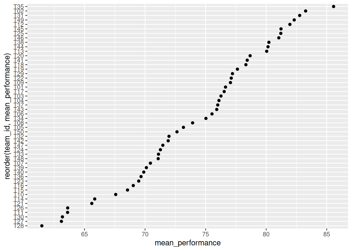
Exercise 9 — multilevel data
empty_model <- lmer ( performance ~ 1 + ( 1 | team_id ) ,
data = teams ,
REML = TRUE
) variance_parts <- as.data.frame ( VarCorr ( empty_model ) ) team_variance <- variance_parts $ vcov [ variance_parts $ grp == "team_id"
] [ 1 ] residual_variance <- sigma ( empty_model ) ^ 2 icc <- team_variance / ( team_variance + residual_variance ) icc multilevel_model <- lmer ( performance ~
engagement + autonomy + workload +
team_climate + manager_support +
( 1 | team_id ) ,
data = teams ,
REML = TRUE
) naive_model <- lm ( performance ~
engagement + autonomy + workload +
team_climate + manager_support ,
data = teams
) coef ( summary ( multilevel_model ) )
                  Estimate Std. Error    t value
(Intercept)     39.1782650  7.1389129  5.4879876
engagement       4.5782124  0.3488634 13.1232254
autonomy         1.9336050  0.3002481  6.4400241
workload        -2.6658346  0.2784960 -9.5722553
team_climate    -0.4101585  1.1912539 -0.3443082
manager_support  3.3436041  1.4257903  2.3450883
                  Estimate Std. Error   t value     Pr(>|t|)
(Intercept)     38.9787383  3.6824357 10.585042 4.192815e-24
engagement       4.6727621  0.4232628 11.039859 6.654828e-26
autonomy         1.8334932  0.3608835  5.080568 5.046686e-07
workload        -2.5971246  0.3311868 -7.841871 2.067436e-14
team_climate    -0.4257966  0.5381656 -0.791200 4.291431e-01
manager_support  3.3371647  0.6275995  5.317347 1.492766e-07
Exercise 10 — scenario analysis
library ( tidyverse ) library ( broom ) retail <- read_csv ( "data/stagnant_retail.csv" , show_col_types = FALSE ) monthly <- retail |> group_by ( month_number ) |>
summarise (
sales = mean ( sales_k_eur ) ,
marketing = mean ( marketing_k_eur ) ,
footfall = mean ( footfall_k ) ,
competitor_pressure = mean ( competitor_pressure ) ,
.groups = "drop"
)
scenario_model <- lm ( sales_k_eur ~
footfall_k +
marketing_k_eur +
discount_pct +
service_quality +
competitor_pressure +
conversion_rate ,
data = retail
) baseline <- retail |> summarise (
footfall_k = median ( footfall_k ) ,
marketing_k_eur = median ( marketing_k_eur ) ,
discount_pct = median ( discount_pct ) ,
service_quality = median ( service_quality ) ,
competitor_pressure = median ( competitor_pressure ) ,
conversion_rate = median ( conversion_rate )
)
student_scenarios <- bind_rows ( baseline |> mutate ( scenario = "Baseline" ) ,
baseline |> mutate (
discount_pct = discount_pct + 3 ,
scenario = "Discount +3 pp"
) ,
baseline |> mutate (
footfall_k = footfall_k * .95 ,
scenario = "Footfall -5%"
)
) pred <- predict ( scenario_model ,
newdata = student_scenarios ,
interval = "confidence"
) |> as.data.frame ( )
bind_cols ( student_scenarios , pred ) |> arrange ( desc ( fit ) )
# A tibble: 3 × 10
  footfall_k marketing_k_eur discount_pct service_quality competitor_pressure
*      <dbl>           <dbl>        <dbl>           <dbl>               <dbl>
1       14.6            25.0        12.4             4.22               0.461
2       14.6            25.0         9.44            4.22               0.461
3       13.8            25.0         9.44            4.22               0.461
# ℹ 5 more variables: conversion_rate <dbl>, scenario <chr>, fit <dbl>,
#   lwr <dbl>, upr <dbl>
These are model-based what-if comparisons, not causal intervention estimates.
Exercise 11 — chi-square
      Finance HR Marketing Operations Technology
  No       70 41        70         97         67
  Yes      27 13        30         28         37
        Finance        HR Marketing Operations Technology
  No  0.2028986 0.1188406 0.2028986  0.2811594  0.1942029
  Yes 0.2000000 0.0962963 0.2222222  0.2074074  0.2740741
    Pearson's Chi-squared test

data:  tab
X-squared = 5.4999, df = 4, p-value = 0.2397
       Finance      HR Marketing Operations Technology
  No  69.71875 38.8125    71.875   89.84375      74.75
  Yes 27.28125 15.1875    28.125   35.15625      29.25
Cramer's V (adj.) |       95% CI
--------------------------------
0.06              | [0.00, 1.00]

- One-sided CIs: upper bound fixed at [1.00].